Notes on Finite Element Method for Cosserat Rod Dynamics
Abstract
This post covers a self-contained Lie group perspective for the modelling of Cosserat rods covering the derivation of the equations of motion using geometric variational calculus, discretization of the equations of motion by a strain parameterization, and a derivation of Implicit and Newmark-beta time stepping schemes.
Introduction
Cosserat rod theory is a beam theory capturing realistic three dimensional of slender continuua and is an important model for soft robotic systems. These systems have drawn strong research interest due to natural compliance with the environment and opportunities for dynamic modeling and simulation (Bensch et al., 2024; Orekhov & Simaan, 2020; Till et al., 2015; Tummers et al., 2023), state estimation (Lilge et al., 2022; Lilge et al., 2024; Zheng et al., 2024), and control (Alqumsan et al., 2019; Doroudchi & Berman, 2021). Soft slender robots have applications in biomedicine, space, and human-robot interaction (Cianchetti et al., 2018; Zhang et al., 2023; Polygerinos et al., 2017).
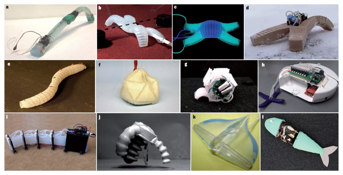
Examples of soft robotic systems (Rus & Tolley, 2015). These notes are meant the be a quick refresher, or introduction to Cosserat rod theory from the modern geometric mechanics perspective (Holm, 2011; Marsden & Ratiu, 1998). In the pursuit to be self-contained, we very briefly review mathematical preliminaries used to derive the equations of motion, this includes the Special Euclidean group and some identities from the calculus from Lie theory (Holm, 2011). We derive the equations of motion first in the Lagrangian formalism, then the equivalent equations of motion in the Hamiltonian formalism and prove some conservation laws. We then use an exact geometric strain parameterization (Boyer et al., 2020; Renda et al., 2020) to discretize the partial differential equations (Grazioso, 2017; Samei, 2022). These notes are self contained, but some ideas are drawn/inspired from the following sources: geometric mechanics (Holm, 2011; Holm et al., 2009; Marsden & Ratiu, 1998), Cosserat theory (Boyer et al., 2010; Boyer et al., 2020; Caasenbrood et al., 2022; Renda et al., 2020; Renda et al., 2018; Renda et al., 2018).
Preliminaries
Special Euclidean Group
The Special Orthogonal group $SO(3)$ is the matrix group of rigid rotations defined by
\[\begin{aligned} SO(3) = \{R \in\mbR^{3\times 3} \, | \, R^T R = I, \quad \det R = 1 \}. \end{aligned}\]with inverse $R^{-1} = R^T$. It’s Lie algebra $\mso(3) \subset \mbR^{3\times 3}$ is the set of all skew-symmetric matrices $\wh{\bOm} + \wh{\bOm} = \bzero$ which can be shown to be tangent space at the identity $\mso(3) = T_{I}SO(3)$ (Holm et al., 2009; Marsden & Ratiu, 1998). There exists an isomorphism $.^\vee:\mso(3) \rightarrow \mbR^3$ defined implicitly $\wh{\bOm}\br = \bOm\times\br$ for any $\br \in \mbR^3$. The hat map $\wh{.}:\mbR^3\rightarrow \mso(3)$ preserves the Lie algebra structure of $(\mbR^3,\times)$,
\[\begin{aligned} \wh{\bOm\times\br} = \wh{\bOm}\wh{\br} - \wh{\br}\wh{\bOm}. \end{aligned}\]The Special Euclidean group $SE(3)$ is the matrix group of all rigid motions (rotation and translations) of $\mbR^3$. It is defined as the semi-direct product $SE(3) = SO(3)\times \mbR^3$ represented by $4\times 4$ matrices
\[\begin{aligned} g = \begin{bmatrix} R & \br\\ \bzero & 1 \end{bmatrix}, \quad g^{-1} = \begin{bmatrix} R^T & -R^T\br\\ \bzero & 1 \end{bmatrix}. \end{aligned}\]The Lie algebra $\mse(3) = \mso(3) \times \mbR^3$ is the set of all twists represented by $4\times 4$ matrices
\[\begin{aligned} \wh{\bX} = \begin{bmatrix} \wh{\bOm}& \bv \\ \bzero & 0 \end{bmatrix}, \quad \wh{\bX}^\vee = \begin{bmatrix} \bOm \\ \bv \end{bmatrix}, \end{aligned}\]where $.^\vee:\mse(3) \rightarrow \mbR^6$ is the inverse hat map for $\mse(3)$ defined in terms of the inverse hat map for $\mso(3)$. For $g = (R,\br) \in SE(3)$, the Adjoint map $\Ad_{g}:\mse(3)^\vee \rightarrow \mse(3)^\vee$ and for $\wh{\bX} \in \mse(3)$, the adjoint map $\ad_{\hat{\bX}}:\mse(3) \rightarrow \mse(3)$ are represented by $6\times 6$ matrices
\[\begin{aligned} [\Ad_{g}] = \begin{bmatrix} R & \mbO\\ \wh{\br}R & R \end{bmatrix}, \quad [\ad_{\wh{\bX}}] = \begin{bmatrix} \wh{\bOm} &\mbO \\ \wh{\bv} & \wh{\bOm} \end{bmatrix} \end{aligned}\]where $\wh{\bX}^\vee = (\bOm,\bv) \in \mbR^6$. Note that the Adjoint with inverse $g^{-1}$ is given by
\[\begin{aligned} & [\Ad_{g^{-1}}] = \begin{bmatrix} R^T & \mbO\\ -R^T\wh{\br} & R^T \end{bmatrix}. \end{aligned}\]The corresponding coAdjoint and coadjoint maps acting on the dual Lie algebra $\mse(3)^*$ are given by
\[\begin{aligned} [\Ad^*_{g}] = \begin{bmatrix} R^T & -R^T\wh{\br} \\ \mbO & R^T \end{bmatrix}, \quad [\ad^{*}_{\wh{\bX}}] = \begin{bmatrix} -\wh{\bOm} & -\wh{\bv} \\ \mbO & -\wh{\bOm} \end{bmatrix} \end{aligned}\]Derivatives of Adjoint Maps
We use these derivatives in the derivation of the equations of motion for the Cosserat rods.
Lemma. For any $g \in SE(3)$ satisfying $\mcV = g^{-1}\pp{g}{t}$, the Adjoint and adjoint maps satisfy the following identities
\[\begin{aligned} &\pp{}{t}\left( \Ad_{g}^{-1}\right) = - \ad_{\mcV}\Ad_{g}^{-1} \\ &\pp{}{t}\left( \Ad_{g}\right) = \Ad_{g}\ad_{\mcV} \\ &\pp{}{t}\left( \Ad_{g^{-1}}^{*}\right) = - \Ad_{g^{-1}}^{*} \ad_{\mcV}^{*} \\ &\pp{}{t}\left( \Ad_{g}^{*}\right) =\ad_{\mcV}^*\Ad_{g}^{*} \end{aligned}\]Proof.
We compute by direct computation, fix a constant vector $\mcW \in \mse(3)$
\[\begin{aligned} \pp{}{t}\Ad_{g}\wh{\mcW} &= \pp{}{t}g\wh{\mcW} g^{-1} =\pp{}{t}g\wh{\mcW} g^{-1} + g\wh{\mcW} \pp{}{t}g^{-1} \\ & = gg^{-1}\dot{g}\wh{\mcW}g^{-1} - g\wh{\mcW}g^{-1}\dot{g}g^{-1} = g\left( \wh{\mcV}\wh{\mcW} - \wh{\mcW}\wh{\mcV}\right)g^{-1}\\ &=\Ad_{g}\ad_{\wh{\mcV}}\wh{\mcW} \end{aligned}\]Similarly, we compute
\[\begin{aligned} \pp{}{t}\Ad_{g^{-1}}\wh{\mcW} &= \pp{}{t}g^{-1}\wh{\mcW} g =-g^{-1}\dot{g}g^{-1}\wh{\mcW} g^{-1} + g^{-1}\wh{\mcW} \dot{g} \\ &=-\wh{\mcV}\Ad_{g^{-1}}\wh{\mcW} + g^{-1}\wh{\mcW}gg^{-1} \dot{g}\\ &=-\left(\wh{\mcV}\Ad_{g^{-1}}\wh{\mcW} - \Ad_{g^{-1}}\wh{\mcW}\wh{\mcV} \right)\\ &-\left[\wh{\mcV},\Ad_{g^{-1}}\wh{\mcW} \right] = -\ad_{\wh{\mcV}}\Ad_{g^{-1}}\wh{\mcW}. \end{aligned}\]For the coadjoint maps, fix any constant $\bPi \in \mse^*(3)$ and any constant $\mcW \in \mse(3)$ and compute
\[\begin{aligned} \aaa{\pp{}{t}\Ad_{g}^{*}\bPi, \mcW} &= \pp{}{t}\aaa{\Ad_{g}^{*}\bPi, \mcW}\\ &= \pp{}{t}\aaa{\bPi, \Ad_{g}\mcW}\\ &= \aaa{\bPi, \pp{}{t}\Ad_{g}\mcW}\\ &= \aaa{\bPi, \Ad_g \ad_\mcV\mcW}\\ &= \aaa{\ad_{\mcV}^{*}\Ad_{g}\bPi,\mcW}. \end{aligned}\]The remaining case is similar.
Lemma. Let $\delta$ be the variational derivative and define $\bpsi = g^{-1}\delta g \in \mse(3)$, then the Adjoint map satisfies
\[\begin{aligned} &\delta \left( \Ad_{g}^{-1}\right) = - \ad_{\bpsi}\Ad_{g}^{-1} \\ &\delta \left( \Ad_{g}\right) = \Ad_{g}\ad_{\bpsi} \\ &\delta\left( \Ad_{g^{-1}}^{*}\right) = - \Ad_{g^{-1}}^{*} \ad_{\bpsi}^{*} \\ &\delta\left( \Ad_{g}^{*}\right) =\ad_{\bpsi}^*\Ad_{g}^{*} \end{aligned}\]Proof.
Similar to the previous lemma, but replace $\delta$ with $\pp{}{t}$ and $\bpsi = g^{-1}\delta g$ with $\mcV = g^{-1}\dot{g}$.
Hamilton’s Variational Principle
Let $Q$ be the configuration space for a simple mechanical system, let $TQ$ be its tangent bundle and let $(\bq,\dot{\bq})$ be its local coordinates. The Lagrangian $L:TQ \rightarrow \mbR$ is defined as the difference of kinetic and potential energies
\[\begin{aligned} L(\bq,\dot{\bq}) = K(\bq,\dot{\bq}) - V(\bq). \end{aligned}\]Let $\bq:[a,b]\rightarrow Q$ be a curve with end points $\bq(a) = \bq_a$, and $\bq(b) = \bq_b$. A variation of this curve is a function $\beta:[a,b]\times\mbR \rightarrow Q$ that matches the end points of the curve $\beta(a,s) = \bq_a$ and $\beta(b,s) = \bq_b$. The variational derivative $\delta$ is defined to be the vector field along the curve $\bq$ given by
\[\begin{aligned} \delta \bq(t) = \pp{\beta(t,s)}{s}\Big|_{s=0} \end{aligned}\]Hamilton’s variational principle is stated as follows
Theorem (Hamilton’s Variational Principle). Let $L:TQ \rightarrow \mbR$ be a Lagrangian function. Then, the (Euler-Lagrange) equations of motion
\[\begin{aligned} -\dd{}{t}\pp{L}{\dot{\bq}} + \pp{L}{\bq} = \bzero \end{aligned}\]for the state evolution $(\bq(t),\dot{\bq}(t))$ satisfies the following variational principle
\[\begin{aligned} 0 = \delta \int^{a}_{b}L(\bq(t),\dot{\bq}(t))\mbox{d}t \end{aligned}\]subject to variations $\delta\bq(t)$ satisfying $\delta\bq(a) =\delta\bq(b) = 0$.
Proof.
\[\begin{aligned} 0 &= \delta \int^{b}_{a}L(\bq(t),\dot{\bq}(t))\mbox{d}t = \int^{b}_{a}\aaa{\pp{L}{\dot{\bq}},\delta\dot{\bq}} + \aaa{\pp{L}{\bq},\delta\bq} \mbox{d} t\\ &= \int^{b}_{a}\aaa{-\dd{}{t}\pp{L}{\dot{\bq}}\mbox{d} t + \pp{L}{\bq}\,, \, \delta \bq} \mbox{d} t + \aaa{\pp{L}{\dot{\bq}},\delta\bq}\Big|_{a}^{b} \end{aligned}\]This equation holds for all variations $\delta\bq(t)$ satisfying $\delta\bq(a) =\delta\bq(b) = 0$. Hence, the left hand side of the product in the integrand must be identically zero.
Cosserat Rod Dynamics
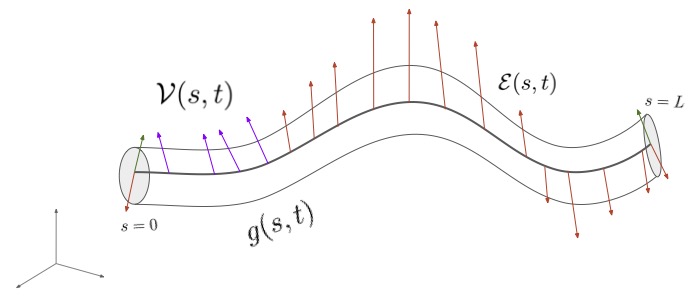
Physically, a Cosserat rod is a 1D model of a beam has three bending modes (two out of plane bending modes, and a twisting modes), and three extension modes (axial, and two sheer modes). Other commonly studied beam models such as the Timoshenko beam and Kirchoff rods may be viewed as special cases of the Cosserat rod. One may also view the Cosserat rod as the continuum limit of an open chain of rigid bodies (a contiuum manipulator).
Lagrangian Formulation
The configuration space for a Cosserat rod of length $L$ is the space of all embedded smooth curves in the Special Euclidean group $\mcQ = {g(s) \in SE(3), \, | \, s\in [0,L]}$. A motion $g(s,t)$ of the rod is a smooth two-parameter hypersurface in $SE(3)$. We define the body (material) frame strain field on the curve to be left translation of the spatial derivative
\[\begin{aligned} \mcE(s,t) = \left(g^{-1}(s,t)\pp{g}{s}(s,t)\right)^\vee = \begin{bmatrix} \bK(s,t) \\ \bGam(s,t) \end{bmatrix} \end{aligned}\]where $\bK(s,t)$ is the angular strain field and $\bGam(s,t)$ is the linear strain field. The body velocity field of the motion is given by
\[\begin{aligned} \mcV(s,t) = \left(g^{-1}(s,t)\pp{g}{t}(s,t)\right)^\vee = \begin{bmatrix} \bOm(s,t) \\ \bV(s,t) \end{bmatrix}, \end{aligned}\]where $\bOm(s,t)$ is the body angular velocity field and $\bV(s,t)$ is the body linear velocity field.
Lemma. The compatibility conditions for a motion $g(s,t)$ to be $C^{2}(SE(3))$ is stated as a differential relationship between the velocity and strain fields
\[\begin{aligned} &\pp{\mcV}{s} = \ad_{\mcV}\mcE + \pp{\mcE}{t}\\ &\pp{^2\mcV}{t\partial s} = \ad_{\pp{\mcV}{t}}\mcE + \ad_{\mcV}\pp{\mcE}{t} + \pp{^2\mcE}{t^2} \end{aligned}\]Proof. A compatibility condition for a motion follows from the commutativity of mixed partial derivatives as follows
\[\begin{aligned} &\pp{g}{s} = g\, \wh{\mcE} \implies \pp{^2 g}{t\partial s} = \pp{g}{t}\wh{\mcE} + g\pp{\wh{\mcE}}{t}\\ &\pp{g}{t} = g\, \wh{\mcV} \implies \pp{^2 g}{s\partial t} = \pp{g}{s}\wh{\mcV} + g\pp{\wh{\mcV}}{s} \end{aligned}\]By equality of mixed partials we have
\[\begin{aligned} \pp{g}{t}\wh{\mcE} + g\pp{\wh{\mcE}}{t} = \pp{g}{s}\wh{\mcV} + g\pp{\wh{\mcV}}{s} \end{aligned}\]and by the definitions of velocity and strain fields we find
\[\begin{aligned} g \wh{\mcE}\wh{\mcV} + g\pp{\wh{\mcV}}{s} = g\wh{\mcV}\wh{\mcE} + g\pp{\wh{\mcE}}{t}. \end{aligned}\]This equation holds for all $g \in SE(3)$, then, we find
\[\begin{aligned} \pp{\wh{\mcV}}{s} = \wh{\mcV}\wh{\mcE} - \wh{\mcE}\wh{\mcV} + \pp{\wh{\mcE}}{t} \end{aligned}\]Then, by the inverse hat map and a time derivative we find the compatibility conditions
\[\begin{aligned} &\pp{\mcV}{s} = \ad_{\mcV}\mcE + \pp{\mcE}{t}\\ &\pp{^2\mcV}{t\partial s} = \ad_{\pp{\mcV}{t}}\mcE + \ad_{\mcV}\pp{\mcE}{t} + \pp{^2\mcE}{t^2} \end{aligned}\]Remark. The compatibility equation is an example of a zero-curvature condition with respect to the Lie-algebra valued connection form
\[\mcB = \mcV dt + \mcE ds.\]Hence, there is a flat relationship between time and spatial variables (Holm, 2011). The Lagrangian for the system is then a function of the form $L(g,\pp{g}{s},\pp{g}{t})$. We say that a Lagrangian density is $SE(3)$ left-invariant if for any $\tl{g} \in SE(3)$ we have
\[\begin{aligned} L_0(\tl{g}\cdot g,\tl{g}\cdot\pp{g}{s},\tl{g}\cdot\pp{g}{t}) = L_0(g,\pp{g}{s},\pp{g}{t}). \end{aligned}\]In particular, choose $\tl{g} = g^{-1}$ and the Lagrangian density written in the body frame $\ell:\mse(3)^{\vee} \rightarrow \mbR$ is given by
\[\begin{aligned} L(\mcV,\mcE) = L_0(\mbI,\left(g^{-1}\pp{g}{t}\right)^{\vee},\left(g^{-1}\pp{g}{s}\right)^{\vee}) \end{aligned}\]in terms of body (material) frame strain $\mcE$ and body frame velocity $\mcV$.
Assumption. We assume that the Lagrangian for the Cosserat rod is left $SE(3)$-invariant. An expression for the (reduced) Lagrangian density under the inverse hat map is given by
\[\begin{aligned} \small L(\mcV,\mcE) = \frac{1}{2}\mcV^{T}\mbM\,\mcV - \frac{1}{2}\left( \mcE - \mcE^{*}\right)^{T}\mbK\,\left( \mcE - \mcE^{*}\right) \end{aligned}\]where $\mbM$ is the constant mass matrix, and $\mbK$ is the constant stiffness matrix both defined per unit length, and $\mcE^*$ is the reference strain. The former defined the total kinetic energy and the later describes the elastic internal energy.
Lemma. Let $\wh{\bpsi} = g^{-1}\delta g \in \mse(3)$ be the variation of the motion $g(s,t)$ induced by the left action of $SE(3)$ i.e., $\delta g = T_{e}L_{g}(\wh{\bpsi}) = g\wh{\bpsi}$. Then, the variations of the velocity and strain fields satisfy
\[\begin{aligned} &\delta\mcV = \pp{\bpsi}{t} + \ad_{\mcV}\bpsi, \quad \delta\mcE = \pp{\bpsi}{s} + \ad_{\mcE}\bpsi. \end{aligned}\]Proof. We calculate
\[\begin{aligned} &\small\delta (g^{-1}\pp{g}{t}) = -g^{-1}\delta g \, g^{-1}\pp{g}{t} + g^{-1}\,\delta \pp{g}{t} = -\wh{\bpsi}\wh{\bOm} + g^{-1}\,\delta \pp{g}{t}\\ &\small \pp{\wh{\bpsi}}{t} = \pp{}{t}(g^{-1}\delta g) = -g^{-1}\pp{g}{t} \, g^{-1}\delta g + g^{-1}\pp{\delta g}{t} = g^{-1}\pp{\delta g}{t} -\wh{\bOm}\wh{\bpsi} \end{aligned}\]Putting these two equations together, we find
\[\begin{aligned} \delta \mcV = \pp{\wh{\bpsi}}{t} + \wh{\bOm}\wh{\bpsi} - \wh{\bpsi}\wh{\bOm}. \end{aligned}\]Therefore, under the inverse hat map we find the expression
\[\begin{aligned} \delta\mcV = \pp{\bpsi}{t} + \ad_{\mcV}\bpsi. \end{aligned}\]Since the role of $s$ in $\mcE$ plays the same role as $t$ in $\mcV$, they result in the expression in. We also assume the work (density) $W_{ext}$ exerted by external force density $\bF_{ext} $ and viscoelastic material $\mbD\dot{\mcE}$ proportional to the time variation of the strain and an active constitutive law $\bF_a(s,t)$. By the principle of virtual work, the variation of the work (density) $\delta W_{ext}$ satisfies
\[\begin{aligned} \small\delta W_{ext} &= \int^{L}_{0}\aaa{\bF_{ext},\psi_{g}} + \aaa{\bLambda_{ext},\delta\mcE_{h}}\, ds \\ & \quad \quad \small + \aaa{\bF_{ext}(0),\bpsi_{g}(0) } - \aaa{\bF_{ext}(L),\bpsi_{g}(L) } \end{aligned}\]where the \emph{external stains} given by $\bLambda_{ext} = -\mbD\pp{\mcE}{t} + \bLambda_a$ are visoelastic strains and actuation inputs.
Theorem (Momentum Strong Cosserat Equations of Motion ). Let $g(s,t) \in Q$ be a motion of a Cosserat rod and let $\mcV(s,t)$ and $\mcE(s,t)$ be its velocity and strain fields respectively. Let the Lagrangian density $L:\mse(3)^\vee\rightarrow \mbR$ be defined by subjected to external work $W_{ext}$ defined by the forces $\bF_{ext}$, a (linear) visoelatic material $\mbB \dot{\mcE}$ and active constitutive law $\bLambda_a$. Then, the strong form of equations of motion are given by
\[\begin{aligned} &\pp{}{t}\bPi -\ad^{*}_{\mcV}\bPi + \pp{}{s}\bLambda_{tot} -\ad^{*}_{\mcE}\bLambda_{tot} = \bF_{ext} \end{aligned}\]where $\bPi = \pp{L}{\mcV} = \mbM\mcV$ is momentum field associated to the velocities $\mcV$, and $\bLambda_{tot} = -\mbK(\mcE - \mcE^*) - \mbD \pp{\mcE}{t} + \bLambda_a$ is the stress field associated to the strain field $\mcE$. These equations are subjected to the following boundary conditions
\[\begin{aligned} \bLambda(0) = -\bF_{ext}(0), \quad \bLambda(L) = \bF_{ext}(L) \end{aligned}\]Furthermore, the motion $g(s,t)$ is reconstructed from the following partial differential equations
\[\begin{aligned} \pp{g}{t} = g\wh{\mcV}, \quad \pp{g}{s} = g\wh{\mcE}. \end{aligned}\]Proof. Let $\wh{\bpsi} = g^{-1}\delta g$ be variations of the motion $g(s,t):[0,1]\times \mbR \rightarrow SE(3)$ that vanish at the boundary:
\[\begin{aligned} \wh{\bpsi}(a,t) = \wh{\bpsi}(b,t) = 0, \quad \text{for all} \, \, t \in \mbR. \end{aligned}\]By Hamilton’s variational principle and Lemma we find
\[\begin{aligned} 0 &= \delta \int^{b}_{a} \int^{L}_{0}L(\mcV(s),\mcE(s)) \mbox{d} s\mbox{d} t + \int^{b}_{a}\delta W_{ext} \mbox{d} t\\ &= \int^{b}_{a} \int^{L}_{0}\aaa{\mbM\mcV,\delta\mcV} + \aaa{-\mbK(\mcE - \mcE^{*}),\delta\mcE}\mbox{d} s\mbox{d} t \\ & + \int^{a}_{b} \int^{L}_{0} \aaa{\bF_{ext},\bpsi} + \aaa{\bLambda_{ext},\delta\mcE}\mbox{d} s\mbox{d} t\\ & + \int^{b}_{a}\aaa{\bF_{ext}(0),\bpsi(0) } - \aaa{\bF_{ext}(L),\bpsi(L) } \, dt\\ &= \int^{b}_{a} \int^{L}_{0}\aaa{\bPi,\pp{\bpsi}{t} + \ad_{\mcE}\bpsi} + \aaa{\bLambda,\pp{\bpsi}{s} + \ad_{\mcV}\bpsi}\mbox{d} s\mbox{d} t\\ & + \int^{b}_{a} \int^{L}_{0} \aaa{\bF_{ext},\bpsi} + \int^{b}_{a}\aaa{\bF_{ext}(0),\bpsi(0) } - \aaa{\bF_{ext}(L),\bpsi(L) }\, dt \end{aligned}\]By the definition of the coAdjoint, integration by parts and the vanishing of the variations at the boundary points, we find
\[\begin{aligned} 0 = &\int^{b}_{a} \int^{L}_{0}\left\langle-\pp{}{t}\bPi + \ad^{*}_{\mcV}\bPi -\pp{}{s}\bLambda_{tot} + \ad^{*}_{\mcE}\bLambda_{tot} +\bF_{ext},\bpsi \right.\Big{\rangle}\mbox{d} s\mbox{d} t \\ & \quad \quad +\int^{b}_{a}\aaa{\bLambda_{tot},\bpsi}\Big|_{0}^{L}\,dt + \int^{b}_{a}\aaa{\bF_{ext}(0),\bpsi(0) } - \aaa{\bF_{ext}(L),\bpsi(L) }\, dt \end{aligned}\]This equation holds for all variations $\bpsi \in \mse(3)^\vee$, therefore the equations of motion are given by
\[\begin{aligned} &-\pp{}{t}\bPi + \ad^{*}_{\mcV}\bPi -\pp{}{s}\bLambda_{tot} + \ad^{*}_{\mcE}\bLambda_{tot} +\bF_{ext} = \bzero, \end{aligned}\]subject to the boundary conditions
\[\begin{aligned} &\bLambda_{tot}(0) = -\bF_{-}\\ &\bLambda_{tot}(L) = \bF_{+}. \end{aligned}\]Theorem (Acceleration Strong Cosserat Equations of Motion ). Let $g(s,t) \in Q$ be a motion of a Cosserat rod and let $\mcV(s,t)$ and $\mcE(s,t)$ be its velocity and strain fields respectively. Let the Lagrangian density $L:\mse(3)^\vee\rightarrow \mbR$ be defined by subjected to external work $\delta W_{ext}$ defined by the forces $\bF_{ext}$ and external strains a (linear) viscoelatic material $\mbD \dot{\mcE}$ and control strains $\bLambda_a = (\bLambda_{\bK},\bLambda_{\bGam})$. Then, the strong form of equations of motion are given by
\[\begin{aligned} &\mbM\begin{bmatrix} \pp{\bOm}{t}\\ \pp{\bV}{t} \end{bmatrix} = -\begin{bmatrix} \wh{\bOm} & \mbO \\ \wh{\bV} & \wh{\bOm} \end{bmatrix}\mbM\begin{bmatrix} \bOm\\ \bV \end{bmatrix} + \left( \pp{}{s} + \begin{bmatrix} \wh{\bK} & \mbO \\ \wh{\bGam} & \wh{\bK} \end{bmatrix}\right) \mbK\begin{bmatrix} \bK - \bK^*\\ \bGam - \bGam^* \end{bmatrix}\\ &-\left( \pp{}{s} + \begin{bmatrix} \wh{\bK} & \mbO \\ \wh{\bGam} & \wh{\bK} \end{bmatrix}\right) \left(-\mbD\begin{bmatrix} \pp{\bK}{t}\\ \pp{\bGam}{t} \end{bmatrix} + \begin{bmatrix} \bLambda_{a\bK}\\ \bLambda_{a\bGam} \end{bmatrix}\right) + \begin{bmatrix} \bF_{\bOm}\\ \bF_{\bV} \end{bmatrix} \end{aligned}\]where $\bF_{ext} = (\bF_{\bOm},\bF_{\bV}) \in \mse(3)^\vee$, $\mcM$ is the mass matrix, $\mbK$ is the elastic stiffness matrix, and $\mbB$ is the viscoelastic dissipation matrix. Furthermore, the motion $g(s,t)$ is reconstructed from the following partial differential equations
\[\begin{aligned} &\pp{R}{t} = R\wh{\bOm}, \quad \pp{R}{s} = R\wh{\bK}\\ &\pp{\br}{t} = R\bV, \quad \pp{\br}{s} = R\bGam. \end{aligned}\]Proof. Follows directly from Theorem, the definition of the Lagrangian density and the (co)adjoint maps.
Theorem. [Conservation Laws] Let $\bPi(s,t) = \pp{L}{\mcV}$ and $\bLambda(s,t) = \pp{L}{\mcE}$ be momentum and stress fields satisfying the Cosserat equations of motion corresponding to a motion $g(s,t) \in SE(3)$. Then, $(\bPi(s,t),\bLambda(s,t))$ satisfy the following conservation law
\[\begin{aligned} &\pp{}{t}\left(\Ad^{*}_{g^{-1}(s,t)} \bPi(s,t)\right) + \pp{}{s}\left(\Ad^{*}_{g^{-1}(s,t)} \bLambda(s,t)\right)\\ & \quad \quad = \Ad^{*}_{g^{-1}(s,t)}\left(\bF_{ext} - \pp{}{s}\left(\mbB\pp{\mcE}{t}\right) +\ad_{\mcE}\left(\mbB\pp{\mcE}{t}\right) \right) \end{aligned}\]for all $t \in \mbR$ and $s\in[0,L]$.
Proof. For any fixed $\eta \in \mse(3)$ we have
\[\begin{aligned} \small &\aaa{\pp{}{t}\Ad^{*}_{g^{-1}}\bPi + \pp{}{s}\Ad^{*}_{g^{-1}}\bLambda,\eta} \\ &= \pp{}{t}\aaa{\Ad^{*}_{g^{-1}}\bPi,\eta} + \pp{}{s}\aaa{\Ad^{*}_{g^{-1}}\bLambda,\eta}\\ &= \pp{}{t}\aaa{\bPi,\Ad_{g^{-1}}\eta} + \pp{}{s}\aaa{\bLambda,\Ad_{g^{-1}}\eta}\\ &= \aaa{\pp{\bPi}{t},\Ad_{g^{-1}}\eta} + \aaa{\bPi,-\ad_{\mcV}\Ad_{g^{-1}}\eta}\\ &\quad +\aaa{\pp{\bLambda}{s},\Ad_{g^{-1}}\eta} + \aaa{\bLambda,-\ad_{\mcE}\Ad_{g^{-1}}\eta} \\ &= \aaa{\Ad^{*}_{g^{-1}} \pp{\bPi}{t}-\Ad^{*}_{g^{-1}}\ad^{*}_{\mcV}\bPi,\eta} \\ &\quad +\aaa{\Ad^{*}_{g^{-1}} \pp{\bLambda}{t}-\Ad^{*}_{g^{-1}}\ad^{*}_{\mcE}\bLambda,\eta} \end{aligned}\]As $(\bPi,\bLambda)$ satisfy the Cosserat equations, we find.
Remark. Theorem may be physically interpreted as follows. The coAdjoint map $\Ad_{g^{-1}}^{*}$ maps the body (material) frame momenta and stress fields into their spatial frame representation. Therefore, can be understood as the total time variation of the momenta field and arclength variation of the stress field is balanced by the total force field on the body represented in the spatial frame. This conservation law is related to circulation in the system (Holm, 2011), and can also be found in the symmetries of charged braids (Ellis et al., 2010).
Hamiltonian Formulation
In this section, we derive the Hamiltonian equations of motion and the associated Poisson bracket. The Hamiltonian formulation of Cosserat rods is an understudied topic which may prove fruitful when further explored as has been the case for other Hamiltonian system. The derivation of the equations is very similar to continuum spin-chains (Holm, 2011) or charged braids (Ellis et al., 2010). Using the Legendre transform, we define the Hamiltonian density function $\mathit{H}:\mfg^{*}\times \mfg \rightarrow \mbR$ given by
\[\begin{aligned} \mathit{H}(\bPi,\mcE) = \aaa{\bPi,\mcV} - L(\mcV,\mcE). \end{aligned}\]Lemma. The relationship between the reduced Lagrangian $L$ and reduced Hamiltonian $\mathit{H}$ and the variables $(\mcV,\mcE)$ and $\bPi$ are stated as
\[\begin{aligned} \mcV = \pp{H}{\mcV}, \quad \bPi = \pp{L}{\mcV}, \quad \pp{H}{\mcE} = -\pp{L}{\mcE} = -\bLambda. \end{aligned}\]Proof. Take the variational derivative of both sides of the Hamiltonian equation
\[\begin{aligned} \delta H &= \aaa{\delta \bPi,\pp{H}{\bPi}} + \aaa{\pp{H}{\mcE},\delta \mcE}\\ &= \delta \left (\aaa{\bPi,\mcV} - L(\mcV,\mcE) \right)\\ &= \aaa{\delta \bPi,\mcV} + \aaa{\bPi - \pp{L}{\mcV},\delta \mcV} - \aaa{\pp{L}{\mcE},\delta \mcE}. \end{aligned}\]Assumption. Assume that the constitutive law is purely elastic: $\mbK\mcE$, i.e., there is no material dependence on the time variation of the strain $\pp{\mcE}{t} = 0$.
Theorem (Hamilton-Cosserat Equations of Motion). Let $\bPi = (\bPi_{\Om},\bPi_{V}) = (\pp{L}{\Om},\pp{L}{V})$ be the momentum field of the beam, and let $\mcE = (\bK,\bGam)$ be its strain field. The Hamiltonian equations of motion for a Cosserat rod subjected to external forces $F_{\bOm}(s,t)$ and $F_{\bV}(s,t)$ are given by
\[\begin{aligned} &\pp{}{t}\begin{bmatrix} \bPi_{\Om}\\ \bPi_{V}\\ \bK \\ \bGam \end{bmatrix} = \begin{bmatrix} \bF_{\Om}\\ \bF_{V}\\ \bzero \\ \bzero \end{bmatrix}+\begin{bmatrix} \bPi_{\Om}\times & \mbO & \pp{}{s}+ \bK\times & \mbO\\ \bPi_{V}\times & \bPi_{\Om}\times & \pp{}{s}+ \bGam\times & \pp{}{s}+ \bGam\times\\ \pp{}{s}+ \bK\times & \pp{}{s}+ \bGam\times & \mbO & \mbO\\ \mbO & \pp{}{s}+ \bK\times & \mbO &\mbO \end{bmatrix} \begin{bmatrix} \pp{H}{\bPi_{\Om}}\\ \pp{H}{\bPi_{V}}\\ \pp{H}{\bK}\\ \pp{H}{\bGam} \end{bmatrix} \end{aligned}\]with reconstruction equations given by
\[\begin{aligned} &\pp{R}{t} = R\wh{\bOm}, \quad \pp{R}{s} = R\wh{\bK}\\ &\pp{\br}{t} = R\bV, \quad \pp{\br}{s} = R\bGam. \end{aligned}\]Proof. The Cosserat-Poincare equations and the compatibility equation we have
\[\begin{aligned} &\pp{}{t}\bPi = \ad_{\mcV}^{*}\bPi -\pp{}{s}\bLambda + \ad_{\mcE}^{*}\bLambda + \bF_{\mcV}\\ &\pp{}{t}\mcE = \pp{}{s}\mcV -\ad_{\mcV}\mcE. \end{aligned}\]Then, substituting the identities for the Hamiltonian we find
\[\begin{aligned} \pp{}{t}\begin{bmatrix} \bPi \\ \mcE \end{bmatrix} = \begin{bmatrix} -\ad_{\bPi}^{*} & \pp{}{s}- \ad_{\mcE}^{*}\\ \pp{}{s} + \ad_{\mcE} & \mbO \end{bmatrix}\begin{bmatrix} \pp{H}{\bPi}\\ \pp{H}{\mcE} \end{bmatrix} + \begin{bmatrix} \bF_{\mcV}\\ \bzero \end{bmatrix} \end{aligned}\]Then using the definitions of the adjoint and coadjoint maps with $\bPi = (\bPi_{\Om},\bPi_{V})$ and $\mcE = (\bK,\bGam)$ we have
\[\begin{aligned} -\ad_{\bPi}^{*} = \begin{bmatrix} \bPi_{\Om}\times & \mbO \\ \bPi_{V}\times & \bPi_{\Om}\times \end{bmatrix}, \quad \ad_{\mcE} = \begin{bmatrix} \bK\times & \bGam\times \\ \mbO & \bK\times \end{bmatrix} \end{aligned}\]we obtain the result.
Discrete Cosserat Rod Equations
### Strain Parameterization The finite element approach based on the strain parameterization is due to or atleast popularized by Boyer and Renda (Boyer et al., 2020; Renda et al., 2018; Renda et al., 2020; Renda et al., 2018). The configuration space for a Cosserat Rod $\mcQ = {g(s):[0,L]\rightarrow SE(3)}$ is the set of all curves of length $L$ embedded into $SE(3)$. These curves satisfy $\dd{g}{s} = g \, \wh{\mcE}$ subject to initial conditions $g_0:= g(0) \in SE(3)$. Define the strain space $\mcS = {\mcE(s):[0,L]\rightarrow \mse(3)}$ as the set of curves of length $L$ embedded in the Lie algebra $\mse(3)$. Physically, this provides a set of twists parameterized by the backbone representing angular and linear strain field. Therefore, the configuration space can be written as a principle bundle $\mcQ \cong SE(3) \times \mcS $ with local coordinates $(g_0,\mcE)$ where $g_0$ describes the rigid motion of the rod and $\mcE$ is the differential strain field. We use the equation in the following lemma for the discreteization of the free Cosserat equations of motion. The lemma relates the time variation of the strain along the rod, to the velocity field of the rod.
Lemma.
Let the initial conditions in the variable $s \in [0,L]$ be given by $g(0,t) = g_{0}(t) \in SE(3)$, which also satisfy
\[\mathcal{V}(0,t) = \mathcal{V}_{0}(t) = g_{0}(t)^{-1}\,\frac{\partial g_{0}(t)}{\partial t}.\]Then the solution to the compatibility equation is
\[\begin{aligned} \mathcal{V}(s,t) = \mathrm{Ad}_{g(s,t)}^{-1}\left(\mathrm{Ad}_{g_0(t)}\mathcal{V}_0(t) + \int_{0}^{s} \mathrm{Ad}_{g(\sigma,t)}\,\frac{\partial \mathcal{E}}{\partial t}(\sigma,t)\,d\sigma\right). \end{aligned}\]Proof. We show that this is a solution to the compatibility equation
\[\begin{aligned} \pp{\mcV}{s} &= \pp{}{s}\left( \Ad_{g(s,t)}^{-1}\left(\Ad_{g_0(t)}\mcV_0(t) + \int^{s}_{0}\Ad_{g(\sigma,t)}\pp{\mcE}{t}(\sigma,t)d\sigma \ \right)\right)\\ &=-\ad_{\mcE}\Ad_{g^{-1}}\left(\Ad_{g_0(t)}\mcV_0(t) + \int^{s}_{0}\Ad_{g(\sigma,t)}\pp{\mcE}{t}(\sigma,t)d\sigma \ \right) \\ &\quad \quad \quad +\Ad_{g^{-1}}\Ad_{g}\pp{\mcE}{t}\\ &= - \ad_{\mcE}\mcV + \pp{\mcE}{t} = \ad_{\mcV}\mcE + \pp{\mcE}{t} \end{aligned}\]and the initial condition is
\[\begin{aligned} \mcV(0,t) = \Ad_{g(0,t)}^{-1}\left(\Ad_{g_0(t)}\mcV_0(t) + \int^{0}_{0}\Ad_{g(\sigma,t)}\pp{\mcE}{t}(\sigma,t)d\sigma \ \right) = \mcV_0. \end{aligned}\]Discrete Kinematics
The velocity field of the system $\mcV(s,t)$ evolves according to, given the evolution of the strain field $\pp{}{t}\mcE$. As such, we approximate the strain field $\mcE$ we separate the $s$ and $t$ variables by specifying $\btheta(t) \in \mbR^{6K}$ shape functions $\bPhi(s) \in \mbR^{6\times 6K}$ whose columns span the strain field
\[\begin{aligned} \mcE(t,s) = \bPhi(s)\btheta(t) + \mcE^*(s) \end{aligned}\]where are strain elements and $\mcE^*(s)$ is the rest strain field value at each $s \in [0,L]$. For any $s \in [L_{K-1},L_{K}]$, by equation $\pp{}{s}g(s,t) = g(s,t)\wh{\mcE}(s,t)$, the configuration of the rod $g(s,t)$ is approximated by
\[\begin{aligned} g(s,t)\! \approx\! g_0(t)\!\circ\!\! \prod^{K-1}_{i=0} \exp(\mathcal{E}(L_{i},t)\Delta s)\!\circ\! \exp(\mathcal{E}(s- L_{K-1},t)), \end{aligned}\]This approximation is a result of Lie-Euler integration which provides a fast computation of the shape of the rod (Samei & Chhabra, 2024).
Shape Variable Examples
Some examples of strain parameterization include, piecewise linear strain (PLS) (Li et al., 2023), for $N$-elements
\[\begin{aligned} \bPhi(s) = \begin{bmatrix} \varphi_1(s)\,\mbI_{6\times6}& \varphi_2(s)\,\mbI_{6\times6} & \dots & \varphi_N(s)\,\mbI_{6\times6} \end{bmatrix} \end{aligned}\]with
\[\begin{aligned} \varphi_i(s) &= \left\{\begin{aligned} & \frac{s- L_{i-1}}{L_i - L_{i-1}}, \quad s \in [L_{i-1},L_{i}]\\ & \frac{L_{i+1}-s}{L_{i+1} - L_{i}}, \quad s \in [L_{i},L_{i+1}]\\ & \quad 0 \quad \quad \quad \quad \quad \text{otherwise} \end{aligned} \right. \end{aligned}\]Legendre polynomials may be used (Caasenbrood et al., 2022) to parameterized
\[\begin{aligned} \bPhi(s) = \mbI_{6\times6}\otimes\begin{bmatrix} \varphi_1(s)& \varphi_2(s)& \dots & \varphi_N(s) \end{bmatrix} \end{aligned}\]where $\varphi_i(s)$ is a Legendre polynomial defined by the following generating function
\[\begin{aligned} \varphi_n(s) = \frac{2}{2^{n}(n-1)!}\dd{^{n-1}}{s^{n-1}}\left( \left(\frac{2s}{L}\right)^{2} - 1\right)^{n-1}, \end{aligned}\]for each $n = 1,\dots,N$, where $N$ is the number of elements.
Discrete Kinematics
Under the strain parameterization and Lemma the velocity of the rod under the discrete strain satisfies
\[\begin{aligned} \mcV(s,t) = \Ad_{g(s,t)}^{-1}\left(\Ad_{g_0(t)}\mcV_0(t) + \int^{s}_{0}\Ad_{g(s,t)}\bPhi(s)d\sigma \dot{\btheta} \ \right). \end{aligned}\]Lemma. Define new velocity variables $\bV = (\mcV_0, \dot{\btheta}) \in \mse(3)^\vee \times \mbR^{6K}$ and Jacobians $\mbJ_{0}$ and $\mbJ_{\theta}$ so that can be written as
\(\begin{aligned} \mcV = \tl{\mbJ}_{0}\mcV_0 + \mbJ_{\theta}\dot{\btheta} = \begin{bmatrix} \tl{\mbJ}_0 & \mbJ_\theta \end{bmatrix}\bV =: \tl{\mbJ}\bV \end{aligned}\)
where the Jacobians \(\tl{\mbJ}_0\) and \(\tl{\mbJ}_{\theta}\) are given by
\[\begin{aligned} & \tl{\mbJ}_0 = \Ad_{g(s,t)}^{-1}\Ad_{ g_0(t)}\\ & \mbJ_{\theta} = \Ad_{g(s,t)^{-1}}\int^{s}_{0}\Ad_{g(\sigma,t)}\bPhi(\sigma)\mbox{d}\sigma. \end{aligned}\]Proof. Follows from. Lemma. The variation of $\bpsi = g^{-1}\delta g \in \mse(3)^\vee$ satisfies
\[\begin{aligned} \bpsi &= \Ad_{g^{-1}(s,t)}\left(\Ad_{g_{0}}\bpsi_{0} + \int^{s}_{0}\Ad_{g(s,t)}\delta \mcE(s,t)d\sigma\right) \\ & = \tl{\mbJ}_{0}\bpsi_0 +\mbJ_{\theta}\delta \btheta \end{aligned}\]where $\bpsi_{0} = g^{-1}(0)\delta g(0) = g^{-1}_{0}\delta g_0$ is the initial condition in variation $s \in [0,L]$ and $\delta \mcE = \bPhi \, \delta \btheta$.
Proof. The variation of $\mcE$ satisfies \(\begin{aligned} \delta \mcE = \pp{\bpsi}{s} + \ad_{\mcE}\bpsi \end{aligned}\)
which we integrate to obtain the result. The previous two lemmas on the Jacobians assume that rigid motion of the base satisfy the following identities
\[\mcV_0 = \left(g_0^{-1}\dot{g}_0 \right)^\vee, \quad \bpsi_0 = \left(g_0^{-1}\delta g_0 \right)^\vee.\]From a numerical implementation perspective, it is much easier to implement a simulation if all the variables are in $\mbR^n$, as many optimization solvers are designed for this space. If we parameterize the rigid motion of the base $g_0(t)$ by a twist $\btheta_0 = \left(\bphi_0,\bp_0 \right)$ we have
\[\begin{aligned} g_0(t) = \begin{bmatrix} R_0(t) & \bp_0(t) \\ \bzero & 1 \end{bmatrix}, \quad R_0(t) = \exp_{SO(3)}(\wh{\bphi}_0(t)). \end{aligned}\]In this parameterization, the (left translated) Jacobian for the rigid velocities $\mcV_0 = \mbJ_{SE(3)}\dot{\btheta}_0$ where the $SE(3)$ Jacobian is
\[\begin{aligned} \mbJ_{SE(3)} = \begin{bmatrix} R_0^T\mbJ_{SO(3)}& \mbO \\ \mbO & R_0^T \end{bmatrix} \end{aligned}\]and the $SO(3)$ Jacobians is
\[\begin{aligned} \mbJ_{SO(3)} = \mbI_{3\times3} + \frac{1 - \cos\norm{\bphi_0}}{\norm{\bphi_0}^2}\wh{\bphi}_0 + \frac{\norm{\bphi_0} - \sin\norm{\bphi_0}}{\norm{\bphi_0}^3}\wh{\bphi}_0^2. \end{aligned}\]Lemma. Define new parameterized variables $\bTheta = (\btheta_0, \dot{\btheta}) \in \mbR^{6(K+1)}$ and Jacobians $\mbJ_{0}$ and $\mbJ_{\theta}$ so that can be written as
\[\begin{aligned} \mcV = \mbJ_{0}\dot{\btheta}_0 + \mbJ_{\theta}\dot{\btheta} = \begin{bmatrix} \mbJ_0 & \mbJ_\theta \end{bmatrix}\dot{\bTheta} =: \mbJ\dot{\bTheta} \end{aligned}\]where the Jacobians $\mbJ_0$ and $\mbJ_{\theta}$ are given by
\[\begin{aligned} & \mbJ_0 = \Ad_{g(s,t)^{-1}}\Ad_{ g_0(t)}\mbJ_{SE(3)}\\ & \mbJ_{\theta} = \Ad_{g(s,t)^{-1}}\int^{s}_{0}\Ad_{g(\sigma,t)}\bPhi(\sigma)\mbox{d}\sigma. \end{aligned}\]Proof. Follows from and the definition of $\mcV_0 = \mbJ_{SE(3)}\dot{\theta}_0$.
Lemma.
The Lie derivatives of the Jacobian, denoted by $\dot{\mbJ}(s,\bTheta)$ along the kinematics is given by
where
\[\begin{aligned} & \dot{\mbJ}_0 = -\ad_{\mcV}\Ad_{g^{-1}\circ g_{0}}\mbJ_{SE(3)} + \Ad_{g^{-1}\circ g_0}\ad_{\mbJ_{SE(3)}\dot{\btheta}_0}\mbJ_{SE(3)} + \Ad_{g^{-1}\circ g_{0}}\dot{\mbJ}_{SE(3)} \\ &\dot{\mbJ}_{\theta} = \Ad_{g}^{-1}\int^{s}_{0}\Ad_{g}\ad_{\mcV}\bPhi(\sigma)d \sigma - \ad_{\mcV}\mbJ_{\theta} \end{aligned}\]Proof. Take a time derivative of $\mbJ(s,\bTheta)$ over the kinematics.
Theorem (Discrete Cosserat Equations). Let $\bTheta = (\btheta_0,\btheta) \in \mbR^{6(N+1)}$ be the strain discretize variables for a Cosserat rod. Then, the discrete Cosserat equations of motion are given by
\[\begin{aligned} &\mcM \ddot{\bTheta} + \mcC(\bTheta, \dot{\bTheta}) \, \dot{\bTheta} + \mcF_{\Theta} = \mcF_{ext} + \mcU_a\\ & g(s,t)\! \approx\! g_0(t)\!\circ\!\! \prod^{K-1}_{i=0} \exp(\mathcal{E}(L_{i},t)\Delta s)\!\circ\! \exp(\mathcal{E}(s- L_{K-1},t)), \quad s \in [L_{K-1},L_K]\\ & \mcE(s,t) = \bPhi(s)\btheta(t) + \mcE^*(s) \end{aligned}\]where the mass matrix is given by
\[\begin{aligned} \mcM = \int^{L}_{0}\mbJ^T \mbM \mbJ \, ds, \end{aligned}\]the Coriolis terms are given by
\[\begin{aligned} \mcC(\bTheta,\dot{\bTheta}) = \int^{L}_{0}\mbJ^T\left(\mbM \dot{\mbJ} - \ad^{T}_{\mbJ \dot{\bTheta}} \mbM \mbJ \right)\, ds, \end{aligned}\]the stiffness and strain damping matrices are
\[\begin{aligned} \mcK = \int^{L}_{0}\bPhi^T \mbK \bPhi \, ds\quad \mcD = \int^{L}_{0}\bPhi^T \mbD \bPhi \, ds \end{aligned}\]defining the elastic forces $\mcF_{\Theta} = (\bzero, -\mcK \btheta - \mcD \dot{\btheta}) \in \mbR^{6}\times \mbR^{6N}$ and the actuation forces
\[\begin{aligned} \mcU_a = \begin{bmatrix} \bzero \\ \int^{L}_{0}\bPhi^T \bLambda_a \, ds \end{bmatrix} \end{aligned}\]and distributed external forces \(\begin{aligned} \mcF_{ext} = \begin{bmatrix} \int^{L}_{0}\mbJ^{T}_{0} \bF_{ext} \, ds \\ \int^{L}_{0}\mbJ^{T}_{\theta} \bF_{ext} \, ds \end{bmatrix}. \end{aligned}\)
Moreover, the system is subject to the following boundary conditions
\[\begin{aligned} &-\mbK\bPhi(0)\btheta - \mbD\bPhi(0)\dot{\btheta} + \mcU_a(0) + \mcF_{-} = 0\\ &-\mbK\bPhi(L)\btheta - \mbD\bPhi(L)\dot{\btheta} + \mcU_a(L) - \mcF_{+} = 0 \end{aligned}\]Proof. First, we note that $\delta \mcV$ in terms of the parameterized variation $\bpsi = \mbJ(s,\bTheta)\delta\bTheta$ is given by
\[\begin{aligned} \delta \mcV = \pp{}{t}\bpsi + \ad_{\mcV}\bpsi = \mbJ\, \begin{bmatrix} \delta\dot{\btheta}_0 \\ \delta \dot{\btheta} \end{bmatrix} + \dot{\mbJ}\, \begin{bmatrix} \delta\btheta_0 \\ \delta\btheta \end{bmatrix} + \ad_{\mbJ \dot{\bTheta}}\, \mbJ\, \begin{bmatrix} \delta\btheta_0 \\ \delta\btheta \end{bmatrix} \end{aligned}\]and $\delta\mcE = \bPhi \delta \btheta$. Then, by Hamilton’s variational principle, we find
\[\begin{aligned} &0 = \int^{b}_{a}\int^{L}_{0}\aaa{\mbM \mcV, \pp{\bpsi}{t} + \ad_{\mcV}\bpsi}dsdt\\ &+\int^{b}_{a}\int^{L}_{0} \aaa{\bF_{ext}, \bpsi}dsdt + \int^{b}_{a}\int^{L}_{0}\aaa{-\mbD\dot{\mcE} + \bLambda_a, \delta \mcE}dsdt \\ &=\small \int^{b}_{a}\int^{L}_{0} \aaa{\mbM\mbJ\dot{\bTheta}, \mbJ\,\begin{bmatrix} \delta\dot{\btheta}_0 \\ \delta\dot{\btheta} \end{bmatrix} + \dot{\mbJ}\, \begin{bmatrix} \delta\btheta_0 \\ \delta\btheta \end{bmatrix} + \ad_{\mbJ \dot{\bTheta}}\, \mbJ\, \begin{bmatrix} \delta\btheta_0 \\ \delta\btheta \end{bmatrix}}dsdt\\ &+\int^{b}_{a}\int^{L}_{0}\aaa{-\mbK \bPhi \btheta - \mbD \bPhi \dot{\btheta}+ \bF_a, \bPhi \delta \btheta}dsdt + \int^{b}_{a}\int^{L}_{0} \aaa{\bF_{ext}, \mbJ \begin{bmatrix} \delta\btheta_0 \\ \delta\btheta \end{bmatrix}}dsdt \\ & = \small \int^{b}_{a}\int^{L}_{0} \aaa{- (\mbJ^T \mbM \mbJ)\ddot{\bTheta} - \mbJ^T\left(\mbM \dot{\mbJ} - \ad_{\mbJ\dot{\bTheta}}^T\mbM \mbJ \right)\dot{\bTheta},\begin{bmatrix} \delta\btheta_0 \\ \delta\btheta \end{bmatrix} }dsdt \\ &\small+ \int^{b}_{a}\int^{L}_{0} \aaa{\begin{bmatrix} \mbJ^{T}_{0}\bF_{ext} \\ -\bPhi^T\mbK\bPhi - \bPhi^T\mbD\bPhi \dot{\btheta} + \bPhi^T\bLambda_a + \mbJ^{T}_{\theta}\bF_{ext} \end{bmatrix}, \begin{bmatrix} \delta\btheta_0 \\ \delta\btheta \end{bmatrix}}dsdt. \end{aligned}\]Note that as we use the variation $\delta \mcE = \bPhi\delta \btheta,$ we do not explicitly integrate by parts to get the bounary terms $\aaa{\bLambda(s,t),\bpsi(s,t)}^{L}_{0}$, thus must insert the boundary condition explicitly
\[\begin{aligned} &\int^{b}_{a}\aaa{\bLambda_{tot}(0) + \bF_{-},\bpsi(0)}dt+ \int^{b}_{a}\aaa{\bLambda_{tot}(L) - \bF_{+},\bpsi(L)}dt\\ &= \int^{b}_{a}\aaa{-\mbK(\mcE(0)- \mcE^{*}(0)) - \mbD\dot{\mcE}(0) + \bLambda_a(0) + \bF_{-},\bpsi(0)}dt\\ &+ \int^{b}_{a}\aaa{-\mbK(\mcE(L)- \mcE^{*}(L)) - \mbD\dot{\mcE}(L) + \bLambda_a(L) - \bF_{+},\bpsi(L)}dt\\ &= \int^{b}_{a}\aaa{-\mbK\bPhi(0)\btheta - \mbD\bPhi(0)\dot{\btheta} + \bLambda_a(0) + \bF_{-},\bpsi(0)}dt\\ &+ \int^{b}_{a}\aaa{-\mbK\bPhi(L)\btheta - \mbD\bPhi(L)\dot{\btheta} + \bLambda_a(L) - \bF_{+},\bpsi(L)}dt \end{aligned}\]Finite Element Method
Implicit Method
The last step set up a numerical simulation of a Cosserat rod is to step the system forward. Let’s now discretize in time steps $\Delta t$ and employ an implicit time stepping scheme of the variables $\bTheta = (\btheta_0,\btheta)$
\[\begin{aligned} & \bTheta_{k} = \bTheta_{k-1} + \Delta t \dot{\bTheta}_{k}\\ & \dot{\bTheta}_{k} = \dot{\bTheta}_{k-1} + \Delta t \ddot{\bTheta}_{k}. \end{aligned}\]From our dynamical equations of motion, we multiply by $\Delta t$ and substitute in the implicit time stepping scheme to find the following set of nonlinear equations
\[\begin{aligned}\left \{ \begin{aligned} & \bTheta_k - \bTheta_{k-1} - \Delta t \dot{\bTheta}_k = \bzero \\ & \left(\mcM_k + \Delta t \mcC_k - \Delta t \mcD \right)\dot{\bTheta}_k - \mcM_{k}\dot{\bTheta}_{k-1} - \Delta t\mcK \bTheta_{k} - \Delta t\left(\mcF_{ext,k} + \mcU_{a,k} \right) = \bzero \\ & -\mbK\bPhi(0)\btheta_k -\mbD\bPhi(0)\dot{\btheta}_k +\mcU_{a,k}(0) +\mcF_{-,k}(0) =\bzero\\ & -\mbK\bPhi(L)\btheta_k -\mbD\bPhi(L)\dot{\btheta}_k +\mcU_{a,k}(L) - \mcF_{+,k}(L)=\bzero \end{aligned}\right. \end{aligned}\]where
\(\mcM_{k} = \mcM(\bTheta_k), \quad \mcC_k = \mcC(\bTheta_k,\dot{\bTheta}_k)\) and any other quantities dependent on $\mbJ(\bTheta)$ and $\dot{\mbJ}(\bTheta,\dot{\bTheta})$ must be integrated at each time step. Therefore, we find at each step $k$ a set of nonlinear equations that must be solved. an algorithm to simulate the dynamics of a Cosserat rod is stated as follows.
- Initial conditions: \(\bTheta_0,\, \dot{\bTheta}_0\), the shape functions \(\bPhi(s)\), external forces \(\bF_{ext}(s,t)\) and active constitutive law \(\bLambda_a(s,t)\), time interval \([0,T_{final}]\) with discrete steps \(\Delta t\).
- For steps \(k=1,2,\dots,K_{final}\), given \((\bTheta_{k-1},\dot{\bTheta}_{k-1})\), form the nonlinear equations by evaluating the Jacobians \(\mbJ(s_i,\bTheta_k)\) and \(\dot{\mbJ}(s_i,\bTheta_k,\dot{\bTheta}_k)\) at a set of Gaussian Quadrature (QP) points \(i=1,\dots,m\), then compute the integrals in \(\mcM,\mcC,\mcF_{ext},\mcU_a\) and the rest using the GQ weights \(w_i\) for \(i=1,\dots,m\) to compute
\(\int^{L}_{0}f(s) ds \approx \sum^{m}_{i=1}w_i f(s_i).\) We repeat the above formulation of the integrals at each step to solve system of equations using gradient descent or Newton-Raphson to obtain the next state $(\bTheta_{k},\dot{\bTheta}_{k})$.
Newmark-Beta
The Newmark beta method (Huang & Jawed, 2019) is a stable time stepping developed to solve Newton’s equations of motion $\mbM \ddot{\bq} + \mbC(\bq,\dot{\bq})\dot{\bq} + \mbN(\bq,\dot{\bq}) = \bF_{ext}$ which reduces energy dissipation due to numerical errors. This Newtonian system is discretized over time step $\Delta t$ by approximating the velocity and acceleration using parameters $\beta \in [0,1/2]$ and $\gamma \in [0,1]$. In the notation $(\bTheta, \dot{\bTheta}, \ddot{\bTheta})$ the discreization of the velocity is given by
\[\begin{aligned} & \dot{\bTheta}_{k} = \dot{\bTheta}_{k-1} + \Delta t\, \ddot{\bTheta}_{\gamma}\\ & \ddot{\bTheta}_{\gamma} = (1-\gamma)\ddot{\bTheta}_{k-1} + \gamma\,\dot{\bTheta}_{k}, \quad \gamma \in [0,1]. \end{aligned}\]The discretization of the position variables (configuration and strain) $\bTheta$ according to this method (mean value theorem)
\[\begin{aligned} &\Theta_{k} = \bTheta_{k-1} + \Delta t, \dot{\bTheta}_{k-1} + \frac{1}{2}\Delta t^2\,\ddot{\bTheta}_{\beta}\\ &\ddot{\bTheta}_{\beta} = (1-2\beta)\ddot{\bTheta}_{k-1} +2\beta \ddot{\bTheta}_{k}, \quad 2\beta \in [0,1]. \end{aligned}\]Combining these equations, we find a system of equations that relates a previous state \((\bTheta_{k-1},\dot{\bTheta}_{k-1}, \ddot{\bTheta}_{k-1})\) to the current state \((\bTheta_{k},\dot{\bTheta}_{k}, \ddot{\bTheta}_{k})\) by solving the system of nonlinear equations
\[\begin{aligned} &\dot{\bTheta}_{k} - \dot{\bTheta}_{k-1} - (1-\gamma)\Delta t\, \ddot{\bTheta}_{k-1} - \gamma \Delta t \ddot{\bTheta}_{k} = \bzero\\ &\bTheta_{k} - \bTheta_{k-1} - \Delta t\, \dot{\bTheta}_{k-1} - \frac{\Delta t^2}{2}\left((1-2\beta)\ddot{\bTheta}_{k-1} + 2\beta \, \ddot{\bTheta}_{k} \right) = \bzero\\ & \mcM_{k}\ddot{\bTheta}_{k} + \mcC_{k}\dot{\bTheta}_{k} + \mcN_{k} - \mcF_{ext,k} = \bzero, \end{aligned}\]where again, at each step $k$, we compute the mass $\mcM_{k}$, Coriolis $\mcC_{k}$, internal $\mcN_{k}$ and external forces and boundary forces $\mcF_{ext,k}$ by numerical integration, such as Gaussian Quadrature. Two common discritization schemes for the parameters $(\beta,\gamma)$ are
- Explicit central difference scheme: $\gamma =1/2$ and $\beta =0$.
- Average constant acceleration: $\gamma = 1/2$ and $\beta = 1/4$.
Conclusion
In these notes we derived the kinematics and dynamics for Cosserat rods using geometric variational calculus. We derived the Lagrangian equations of motion and their equivalent Hamiltonian equations of motion. We discretized the Lagrangian formulation using a strain parameterization. Finally, we showed an algorithm to simulate the dynamics using an implicit discretization and Newmark-beta schemes. In future work, we perform and study numerical simulations of the Cosserat equations, including examining locomotion for such systems. Parallelizing the computations of the Jacobians and other quantities might speed up performance. Physics informed Neural networks for simulation and control is another interesting direction. Locomotion is a result of the interaction with the rods environment, which may include coulomb contact forces (Xun et al., 2024) for crawling for slithering, or locomotion could result from the interaction of the rod with hydrodynamic forces resulting in swimming (Boyer et al., 2010).
References
- Bensch, M., Job, T.-D., Habich, T.-L., Seel, T., & Schappler, M. (2024). Physics-Informed Neural Networks for Continuum Robots: Towards Fast Approximation of Static Cosserat Rod Theory. 2024 IEEE International Conference on Robotics and Automation (ICRA), 17293–17299.
- Orekhov, A. L., & Simaan, N. (2020). Solving cosserat rod models via collocation and the magnus expansion. 2020 IEEE/RSJ International Conference on Intelligent Robots and Systems (IROS), 8653–8660.
- Till, J., Bryson, C. E., Chung, S., Orekhov, A., & Rucker, D. C. (2015). Efficient computation of multiple coupled Cosserat rod models for real-time simulation and control of parallel continuum manipulators. 2015 IEEE International Conference on Robotics and Automation (ICRA), 5067–5074.
- Tummers, M., Lebastard, V., Boyer, F., Troccaz, J., Rosa, B., & Chikhaoui, M. T. (2023). Cosserat rod modeling of continuum robots from newtonian and lagrangian perspectives. IEEE Transactions on Robotics, 39(3), 2360–2378.
- Lilge, S., Barfoot, T. D., & Burgner-Kahrs, J. (2022). Continuum robot state estimation using Gaussian process regression on SE (3). The International Journal of Robotics Research, 41(13-14), 1099–1120.
- Lilge, S., Barfoot, T. D., & Burgner-Kahrs, J. (2024). State estimation for continuum multi-robot systems on SE (3). IEEE Transactions on Robotics.
- Zheng, T., McFarland, C., Coad, M., & Lin, H. (2024). Estimating infinite-dimensional continuum robot states from the tip. 2024 IEEE 7th International Conference on Soft Robotics (RoboSoft), 572–578.
- Alqumsan, A. A., Khoo, S., & Norton, M. (2019). Robust control of continuum robots using Cosserat rod theory. Mechanism and Machine Theory, 131, 48–61.
- Doroudchi, A., & Berman, S. (2021). Configuration tracking for soft continuum robotic arms using inverse dynamic control of a Cosserat rod model. 2021 IEEE 4th International Conference on Soft Robotics (RoboSoft), 207–214.
- Cianchetti, M., Laschi, C., Menciassi, A., & Dario, P. (2018). Biomedical applications of soft robotics. Nature Reviews Materials, 3(6), 143–153.
- Zhang, Y., Li, P., Quan, J., Li, L., Zhang, G., & Zhou, D. (2023). Progress, challenges, and prospects of soft robotics for space applications. Advanced Intelligent Systems, 5(3), 2200071.
- Polygerinos, P., Correll, N., Morin, S. A., Mosadegh, B., Onal, C. D., Petersen, K., Cianchetti, M., Tolley, M. T., & Shepherd, R. F. (2017). Soft robotics: Review of fluid-driven intrinsically soft devices; manufacturing, sensing, control, and applications in human-robot interaction. Advanced Engineering Materials, 19(12), 1700016.
- Rus, D., & Tolley, M. T. (2015). Design, fabrication and control of soft robots. Nature, 521(7553), 467–475.
- Holm, D. D. (2011). Geometric Mechanics-Part II: Rotating, Translating and Rolling. World Scientific.
- Marsden, J. E., & Ratiu, T. S. (1998). Introduction to mechanics and symmetry.
- Boyer, F., Lebastard, V., Candelier, F., & Renda, F. (2020). Dynamics of continuum and soft robots: A strain parameterization based approach. IEEE Transactions on Robotics, 37(3), 847–863.
- Renda, F., Armanini, C., Lebastard, V., Candelier, F., & Boyer, F. (2020). A geometric variable-strain approach for static modeling of soft manipulators with tendon and fluidic actuation. IEEE Robotics and Automation Letters, 5(3), 4006–4013.
- Grazioso, S. (2017). Geometric soft robotics: a finite element approach.
- Samei, H. M. (2022). Geometric Recursive Dynamic Modelling and Simulation of Soft Robotic Systems [PhD thesis]. Carleton University.
- Holm, D. D., Schmah, T., & Stoica, C. (2009). Geometric mechanics and symmetry: from finite to infinite dimensions (Vol. 12). Oxford University Press.
- Boyer, F., Porez, M., & Leroyer, A. (2010). Poincaré–Cosserat equations for the Lighthill three-dimensional large amplitude elongated body theory: application to robotics. Journal of Nonlinear Science, 20, 47–79.
- Caasenbrood, B., Pogromsky, A., & Nijmeijer, H. (2022). Energy-shaping controllers for soft robot manipulators through port-hamiltonian cosserat models. SN Computer Science, 3(6), 494.
- Renda, F., Giorgio-Serchi, F., Boyer, F., Laschi, C., Dias, J., & Seneviratne, L. (2018). A unified multi-soft-body dynamic model for underwater soft robots. The International Journal of Robotics Research, 37(6), 648–666.
- Renda, F., Boyer, F., Dias, J., & Seneviratne, L. (2018). Discrete cosserat approach for multisection soft manipulator dynamics. IEEE Transactions on Robotics, 34(6), 1518–1533.
- Ellis, D. C. P., Gay-Balmaz, F., Holm, D. D., Putkaradze, V., & Ratiu, T. S. (2010). Symmetry reduced dynamics of charged molecular strands. Archive for Rational Mechanics and Analysis, 197, 811–902.
- Samei, H., & Chhabra, R. (2024). SuRFR: A fast recursive simulator for soft manipulators with discrete joints on SE (3). Mechanism and Machine Theory, 194, 105589.
- Li, H., Xun, L., & Zheng, G. (2023). Piecewise linear strain cosserat model for soft slender manipulator. IEEE Transactions on Robotics, 39(3), 2342–2359.
- Huang, W., & Jawed, M. K. (2019). Newmark-beta method in discrete elastic rods algorithm to avoid energy dissipation. Journal of Applied Mechanics, 86(8), 084501.
- Xun, L., Zheng, G., & Kruszewski, A. (2024). Cosserat-Rod Based Dynamic Modeling of Soft Slender Robot Interacting with Environment. IEEE Transactions on Robotics.
Enjoy Reading This Article?
Here are some more articles you might like to read next: