Notes on Finite Difference Method for Cosserat Rod Dynamics
Abstract
These are notes on a finite-difference method for Cosserat rod dynamics, including the geometric formulation of the PDEs and shooting-method boundary value solvers.
Introduction
Cosserat rods are an important model for soft slender robotic systems such as continuum manipulators. These systems have drawn research interest due to natural compliance with the environment and opportunities for dynamic modeling and numerical simulation (Bensch et al., 2024; Orekhov & Simaan, 2020; Till et al., 2015; Tummers et al., 2023), state estimation (Lilge et al., 2022; Lilge et al., 2024; Zheng et al., 2024), and control (Alqumsan et al., 2019; Doroudchi & Berman, 2021). Soft slender robots have applications in biomedicine (Cianchetti et al., 2018), mobile robotics (Zhang et al., 2023), and human-robot interaction (Polygerinos et al., 2017).
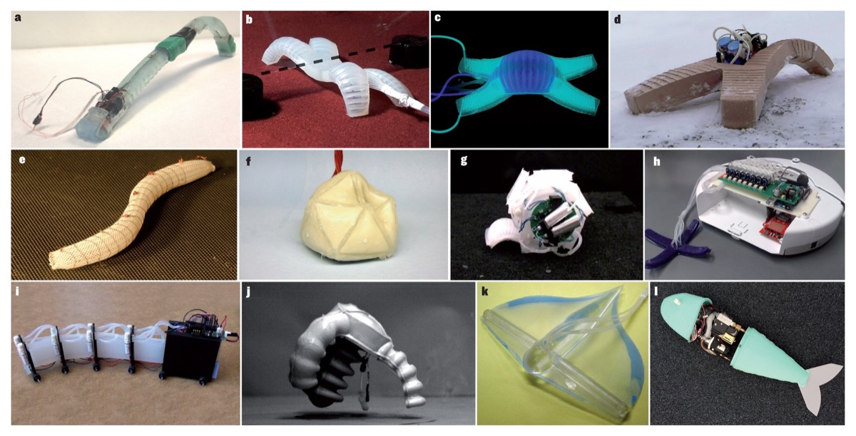
Examples of soft robotic systems (Rus & Tolley, 2015).
These notes are meant as a quick refresher on Cosserat rod theory from a geometric mechanics perspective (Holm, 2011; Marsden & Ratiu, 1998). To stay self-contained, we briefly review preliminaries on the Special Euclidean group and Lie-theoretic identities (Holm, 2011). We then state the strong-form equations of motion and derive a finite-difference discretization in time, followed by boundary value formulations solved with shooting methods (Grazioso, 2017; Samei, 2022; Till et al., 2015). Background sources include geometric mechanics (Holm, 2011; Holm et al., 2009; Marsden & Ratiu, 1998) and Cosserat theory (Boyer et al., 2010; Boyer et al., 2020; Caasenbrood et al., 2022; Renda et al., 2020; Renda et al., 2018; Renda et al., 2018).
Preliminaries
To keep these notes self-contained, we review rigid motion groups and the strong form of dynamic Cosserat equations using Lie group theory.
Special Euclidean Group
Rigid Rotations. The Special Orthogonal group $SO(3)$ is
\[\begin{aligned} SO(3) = \{R \in\mbR^{3\times 3} \, | \, R^T R = I, \quad \det R = 1 \}. \end{aligned}\]Its inverse is $R^{-1} = R^T$. Its Lie algebra $\mso(3) \subset \mbR^{3\times 3}$ is the set of skew-symmetric matrices, and can be identified with $T_I SO(3)$ (Holm et al., 2009; Marsden & Ratiu, 1998). The hat map preserves Lie algebra structure:
\[\begin{aligned} \wh{\bOm\times\br} = \wh{\bOm}\wh{\br} - \wh{\br}\wh{\bOm}. \end{aligned}\]Rigid Motion. The Special Euclidean group $SE(3) = SO(3)\times\mbR^3$ is represented by
\[\begin{aligned} g = \begin{bmatrix} R & \br\\ \bzero & 1 \end{bmatrix}, \quad g^{-1} = \begin{bmatrix} R^T & -R^T\br\\ \bzero & 1 \end{bmatrix}. \end{aligned}\]Its Lie algebra $\mse(3)=\mso(3)\times\mbR^3$ can be represented as
\[\begin{aligned} \wh{\bX} = \begin{bmatrix} \wh{\bOm}& \bv \\ \bzero & 0 \end{bmatrix}, \quad \wh{\bX}^\vee = \begin{bmatrix} \bOm \\ \bv \end{bmatrix}. \end{aligned}\]For $g=(R,\br)\in SE(3)$ and $\wh{\bX}\in\mse(3)$:
\[\begin{aligned} [\Ad_g] = \begin{bmatrix} R & \wh{\br}R \\ \mbO & R \end{bmatrix}, \quad [\ad_{\wh{\bX}}] = \begin{bmatrix} \wh{\bOm} & \wh{\bv} \\ \mbO & \wh{\bOm} \end{bmatrix}. \end{aligned}\]The coAdjoint and coadjoint maps are
\[\begin{aligned} [\Ad_g^*] = \begin{bmatrix} R^T & \mbO \\ -R^T\wh{\br} & R^T \end{bmatrix}, \quad [\ad_{\wh{\bX}}^*] = \begin{bmatrix} -\wh{\bOm} & \mbO \\ -\wh{\bv} & -\wh{\bOm} \end{bmatrix}. \end{aligned}\]Cosserat Rod Dynamics
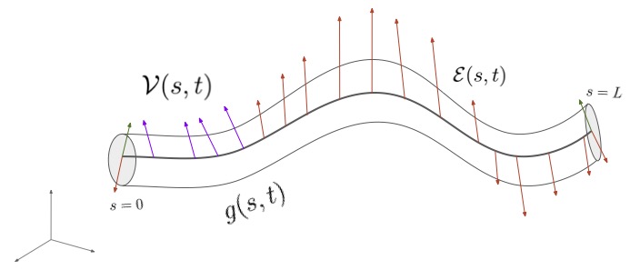
The configuration space for a rod of length $L$ is $\mcQ = {g(s)\in SE(3)\,|\,s\in[0,L]}$. A motion $g(s,t)$ is a smooth two-parameter surface in $SE(3)$. The body-frame strain field is
\[\begin{aligned} \mcE(s,t) = \left(g^{-1}(s,t)\pp{g}{s}(s,t)\right)^\vee = \begin{bmatrix} \bK(s,t) \\ \bGam(s,t) \end{bmatrix}, \end{aligned}\]and the body velocity field is
\[\begin{aligned} \mcV(s,t) = \left(g^{-1}(s,t)\pp{g}{t}(s,t)\right)^\vee = \begin{bmatrix} \bOm(s,t) \\ \bV(s,t) \end{bmatrix}. \end{aligned}\]Lemma. The compatibility condition for $g(s,t)\in C^2(SE(3))$ is
\[\begin{aligned} \pp{\mcV}{s} = \ad_{\mcV}\mcE + \pp{\mcE}{t}. \end{aligned}\]Proof. Follows by a direct computation from commutativity of mixed partial derivatives.
A reduced Lagrangian density is
\[\begin{aligned} L(\mcV,\mcE)=\frac{1}{2}\mcV^T\mbM(s)\mcV -\left(\mcE-\mcE^*\right)^T\mbK(s)\left(\mcE-\mcE^*\right), \end{aligned}\]where $\mbM$ is the mass matrix per unit length, $\mbK$ is the stiffness matrix per unit length, and $\mcE^*$ is the reference strain.
Lemma. Let $\wh{\bpsi}=g^{-1}\delta g\in\mse(3)$. Then
\[\begin{aligned} \delta\mcV = \pp{\bpsi}{t} + \ad_{\mcV}\bpsi, \quad \delta\mcE = \pp{\bpsi}{s} + \ad_{\mcE}\bpsi. \end{aligned}\]Proof. A straightforward computation.
Assuming external force density $\bF_{ext}$, viscoelastic strain term $\mbD\dot{\mcE}$, and active constitutive law $\bLambda_a$, the virtual work variation is
\[\begin{aligned} \delta W_{ext} &= \int_0^L \aaa{\bF_{ext},\psi_g} + \aaa{\bLambda_{ext},\delta\mcE_h}\,ds \\ &\quad + \aaa{\bF_{ext,BC}(0),\bpsi_g(0)} - \aaa{\bF_{ext,BC}(L),\bpsi_g(L)}, \end{aligned}\]with $\bLambda_{ext}=\mbD\pp{\mcE}{t}+\bLambda_a$.
Theorem (Strong Cosserat Equations of Motion). Let $g(s,t)$ be a rod motion with fields $\mcV(s,t)$ and $\mcE(s,t)$, with external work from $\bF_{ext}$, viscoelastic material term, and active constitutive law. The strong-form PDEs are
\[\begin{aligned} &\pp{}{s}g = g\wh{\mcE}, \quad \pp{}{t}g = g\wh{\mcV}, \\ &\pp{}{s}\mcV = \pp{}{t}\mcE + \ad_{\mcV}\mcE, \\ &\pp{}{s}\bLambda = \pp{}{t}(\mbM\mcV) - \ad^*_{\mcV}\mbM\mcV + \ad^*_{\mcE}\bLambda - \bF_{ext}, \end{aligned}\]where
\[\begin{aligned} \bLambda = \mbK(\mcE-\mcE^*) + \mbD\pp{\mcE}{t} + \bLambda_a. \end{aligned}\]Boundary conditions are either:
- Cantilevered boundary conditions:
- Free-free boundary conditions:
Proof. Follows from Hamilton’s variational principle.
Finite Difference Method
For the two-parameter Cosserat PDEs, time derivatives are discretized with a second-order backward difference:
\[\begin{aligned} \pp{}{t}\mcE(s,t) &\approx \frac{1}{\Delta t}\left(\frac{3}{2}\mcE(s,t)-2\mcE(s,t-\Delta t)+\frac{1}{2}\mcE(s,t-2\Delta t)\right), \\ \pp{}{t}\mcV(s,t) &\approx \frac{1}{\Delta t}\left(\frac{3}{2}\mcV(s,t)-2\mcV(s,t-\Delta t)+\frac{1}{2}\mcV(s,t-2\Delta t)\right). \end{aligned}\]Define
\[\begin{aligned} \pp{}{t}\mcE(s,t) &\approx c_0\mcE(s,t)+\mcE^h(s,t), \\ \pp{}{t}\mcV(s,t) &\approx c_0\mcV(s,t)+\mcV^h(s,t), \\ c_0&=\frac{3}{2\Delta t},\quad c_1=-\frac{2}{\Delta t},\quad c_2=\frac{1}{2\Delta t}. \end{aligned}\]Then the semi-discrete system in space is
\[\begin{aligned} &\pp{}{s}g = g\wh{\mcE}, \\ &\pp{}{s}\mcV = c_0\mcE(s,t)+\mcE^h(s,t)+\ad_{\mcV}\mcE, \\ &\pp{}{s}\bLambda = \mbM\left(c_0\mcV(s,t)+\mcV^h(s,t)\right)-\ad^*_{\mcV}\mbM\mcV+\ad^*_{\mcE}\bLambda-\bF_{ext}, \\ &\mcE(s,t)=\left(\mbK+c_0\mbD\right)^{-1}\left(\bLambda-\bLambda_a+\mbK\mcE^*(s)-\mbD\mcE^h(s,t)\right). \end{aligned}\]with either cantilevered or free-free boundary conditions as above.
Boundary Value Problem
Cantilevered B.C.
For the cantilevered case, at each time step $t$ we are given tip boundary force $F_{BC,L}(t)$ and initial conditions $g_0(t)$, $\mcV_0(t)$. We solve for an initial stress guess by minimizing
\[\begin{aligned} \mcL = ||\bLambda_{integrated}(g_0,\mcV_0,\bLambda_{0,guess}) - \bF_{BC,L}||^2. \end{aligned}\]Here, shooting means optimizing a guess of initial conditions $(g_0(t),\mcV_0(t),\bLambda(0,t))$ and integrating so that $\bLambda(L,t)=\bF_{BC,L}(t)$ is satisfied. The optimization can be solved with Levenberg-Marquardt.
Free-Free Boundary Conditions
For free-free conditions, both endpoints are free. We parameterize the base point $g(0)=g_0=(R_0,\br_0)\in SO(3)\times\mbR^3$ and solve for it at each step. Assuming step-$n$ states are known, we apply a Newmark-beta update (Boyer et al., 2022):
\[\begin{aligned} \br_{0,n+1} &= a\ddot{\br}_{0,n+1}+\bff_n, \\ \dot{\br}_{0,n+1} &= b\ddot{\br}_{0,n+1}+\bh_n, \end{aligned}\]with
\[\begin{aligned} a &= \beta\Delta t^2, \quad b=\beta\Delta t^2, \\ \bff_n &= \br_{0,n}+\Delta t\dot{\br}_{0,n}+\Delta t^2\left(\frac{1}{2}-\beta\right)\ddot{\br}_{0,n}, \\ \bh_n &= \dot{\br}_{0,n}+\Delta t(1-\gamma)\ddot{\br}_{0,n}. \end{aligned}\]Rotation updates are
\[\begin{aligned} \bTheta_{0,n+1} &= a\dot{\bOm}_{0,n+1}+\boldsymbol{k}_n, \quad \bOm_{0,n+1}=b\dot{\bOm}_{0,n+1}+\boldsymbol{l}_n, \\ \boldsymbol{k}_n &= \Delta t\bOm_{0,n}+\Delta t^2\left(\frac{1}{2}-\beta\right)\dot{\bOm}_{0,n}, \quad \boldsymbol{l}_n=\bOm_{0,n}+\Delta t(1-\gamma)\dot{\bOm}_{0,n}, \end{aligned}\]and
\[\begin{aligned} R_{0,n+1}=R_{0,n}\exp(\wh{\bTheta}_{0,n+1}). \end{aligned}\]Kinematic relations:
\[\begin{aligned} g_0 &= \begin{bmatrix} R_0\exp(\wh\bTheta_0) & \br_0 \\ \bzero & 1 \end{bmatrix}, \\ \mcV_0 &= \begin{bmatrix} \bOm_0 \\ R_0^T\dot{\br}_0 \end{bmatrix}, \\ \dot{\mcV}_0 &= \begin{bmatrix} \dot{\bOm}_0 \\ R_0^T\ddot{\br}_0 + (R_0^T\dot{\br}_0)\times\bOm_0 \end{bmatrix}. \end{aligned}\]Parameterizing $\bphi_0=(\bTheta_0,\br_0)\in\mbR^6$:
\[\begin{aligned} g_0=\mbA(\bphi_0), \quad \dot{\mcV}_0=\mbB(\bphi_0), \quad \dot{\mcV}_0=\mbC(\bphi_0). \end{aligned}\]with
\[\begin{aligned} \mbA(\bphi_0) &= \begin{bmatrix} R_0\exp(\wh\bTheta_0) & \br_0 \\ \bzero & 1 \end{bmatrix}, \\ \mbB(\bphi_0) &= \begin{bmatrix} \tl{a}\bTheta_0+\tl{\boldsymbol{k}}_n \\ R_0^T(\tl{b}\br_0+\tl{\boldsymbol{h}}_n) \end{bmatrix}, \\ \mbC(\bphi_0) &= \begin{bmatrix} \tl{b}\bTheta_0+\tl{\boldsymbol{l}}_n \\ R_0^T(\tl{b}\br_0+\tl{\boldsymbol{h}}_n)+\bV_0\times\bOm_0 \end{bmatrix}. \end{aligned}\]Parameters:
\[\begin{aligned} R_0^T &= \exp(\wh\bTheta_0)R_{0,n}^T, \quad \tl{b}=a^{-1}, \quad \tl{a}=b\tl{b}, \\ \tl{\boldsymbol{h}}_n &= -b\bff_n, \quad \tl\bff_n = \boldsymbol{h}_n-\tl{a}\bff_n, \\ \tl{\boldsymbol{l}}_n &= -\tl{b}\boldsymbol{k}_n, \quad \tl{\boldsymbol{k}}_n = \boldsymbol{l}_n-\tl{a}\boldsymbol{k}_n. \end{aligned}\]Jacobians:
\[\begin{aligned} \pp{\mbA}{\bphi_0} &= \begin{bmatrix} T(\bTheta_0) & \bzero \\ \bzero & R_0^T \end{bmatrix}, \\ \pp{\mbB}{\bphi_0} &= \begin{bmatrix} \tl{a}\mbI_{3\times 3} & \mbO \\ \wh\bV_0T(\bTheta_0) & \tl{a}R_0^T \end{bmatrix}, \\ \pp{\mbC}{\bphi_0} &= \begin{bmatrix} \tl{b}\mbI_{3\times 3} & \mbO \\ \left(\wh{\bA}_0-\wh{\bOm}_0\wh{\bV}_0\right)T(\bTheta_0)+\tl{a}\wh{\bV}_0 & \left(\tl{b}\mbI_{3\times 3}-\tl{a}\wh{\bOm}_0\right)R_0^T \end{bmatrix}. \end{aligned}\]where \(\bA_0=\dot{\bV}_0+\bOm_0\times\bV_0$ and $(R_0^T\Delta R_0)^\vee=T(\bTheta_0)\Delta\bTheta_0\). At each time step, with base and tip boundary forces $F_{BC,0}(t),F_{BC,L}(t)$, we solve
\[\begin{aligned} \mcL = ||\bLambda_{integrated}(\bphi_{0,guess}) - \bF_{BC,L}||^2, \end{aligned}\]using Levenberg-Marquardt.
Its worth mentioning that the FDM for free-free boundary conditions is very sensitive to the time and spatial integration, making it difficult to converge to the true solution.
Conclusion
These notes reviewed Cosserat rod equations and finite-difference simulation in a Lie-group representation. We stated cantilevered and free-free boundary value problems and outlined shooting-method solutions. Future work includes stronger free-free formulations, contact-force models (Xun et al., 2023), and numerical stability analysis for finite-difference schemes in soft robotic systems (Boyer et al., 2022).
References
- Bensch, M., Job, T.-D., Habich, T.-L., Seel, T., & Schappler, M. (2024). Physics-Informed Neural Networks for Continuum Robots: Towards Fast Approximation of Static Cosserat Rod Theory. 2024 IEEE International Conference on Robotics and Automation (ICRA), 17293–17299.
- Orekhov, A. L., & Simaan, N. (2020). Solving cosserat rod models via collocation and the magnus expansion. 2020 IEEE/RSJ International Conference on Intelligent Robots and Systems (IROS), 8653–8660.
- Till, J., Bryson, C. E., Chung, S., Orekhov, A., & Rucker, D. C. (2015). Efficient computation of multiple coupled Cosserat rod models for real-time simulation and control of parallel continuum manipulators. 2015 IEEE International Conference on Robotics and Automation (ICRA), 5067–5074.
- Tummers, M., Lebastard, V., Boyer, F., Troccaz, J., Rosa, B., & Chikhaoui, M. T. (2023). Cosserat rod modeling of continuum robots from newtonian and lagrangian perspectives. IEEE Transactions on Robotics, 39(3), 2360–2378.
- Lilge, S., Barfoot, T. D., & Burgner-Kahrs, J. (2022). Continuum robot state estimation using Gaussian process regression on SE (3). The International Journal of Robotics Research, 41(13-14), 1099–1120.
- Lilge, S., Barfoot, T. D., & Burgner-Kahrs, J. (2024). State estimation for continuum multi-robot systems on SE (3). IEEE Transactions on Robotics.
- Zheng, T., McFarland, C., Coad, M., & Lin, H. (2024). Estimating infinite-dimensional continuum robot states from the tip. 2024 IEEE 7th International Conference on Soft Robotics (RoboSoft), 572–578.
- Alqumsan, A. A., Khoo, S., & Norton, M. (2019). Robust control of continuum robots using Cosserat rod theory. Mechanism and Machine Theory, 131, 48–61.
- Doroudchi, A., & Berman, S. (2021). Configuration tracking for soft continuum robotic arms using inverse dynamic control of a Cosserat rod model. 2021 IEEE 4th International Conference on Soft Robotics (RoboSoft), 207–214.
- Cianchetti, M., Laschi, C., Menciassi, A., & Dario, P. (2018). Biomedical applications of soft robotics. Nature Reviews Materials, 3(6), 143–153.
- Zhang, Y., Li, P., Quan, J., Li, L., Zhang, G., & Zhou, D. (2023). Progress, challenges, and prospects of soft robotics for space applications. Advanced Intelligent Systems, 5(3), 2200071.
- Polygerinos, P., Correll, N., Morin, S. A., Mosadegh, B., Onal, C. D., Petersen, K., Cianchetti, M., Tolley, M. T., & Shepherd, R. F. (2017). Soft robotics: Review of fluid-driven intrinsically soft devices; manufacturing, sensing, control, and applications in human-robot interaction. Advanced Engineering Materials, 19(12), 1700016.
- Rus, D., & Tolley, M. T. (2015). Design, fabrication and control of soft robots. Nature, 521(7553), 467–475.
- Holm, D. D. (2011). Geometric Mechanics-Part II: Rotating, Translating and Rolling. World Scientific.
- Marsden, J. E., & Ratiu, T. S. (1998). Introduction to mechanics and symmetry.
- Grazioso, S. (2017). Geometric soft robotics: a finite element approach.
- Samei, H. M. (2022). Geometric Recursive Dynamic Modelling and Simulation of Soft Robotic Systems [PhD thesis]. Carleton University.
- Holm, D. D., Schmah, T., & Stoica, C. (2009). Geometric mechanics and symmetry: from finite to infinite dimensions (Vol. 12). Oxford University Press.
- Boyer, F., Porez, M., & Leroyer, A. (2010). Poincaré–Cosserat equations for the Lighthill three-dimensional large amplitude elongated body theory: application to robotics. Journal of Nonlinear Science, 20, 47–79.
- Boyer, F., Lebastard, V., Candelier, F., & Renda, F. (2020). Dynamics of continuum and soft robots: A strain parameterization based approach. IEEE Transactions on Robotics, 37(3), 847–863.
- Caasenbrood, B., Pogromsky, A., & Nijmeijer, H. (2022). Energy-shaping controllers for soft robot manipulators through port-hamiltonian cosserat models. SN Computer Science, 3(6), 494.
- Renda, F., Armanini, C., Lebastard, V., Candelier, F., & Boyer, F. (2020). A geometric variable-strain approach for static modeling of soft manipulators with tendon and fluidic actuation. IEEE Robotics and Automation Letters, 5(3), 4006–4013.
- Renda, F., Giorgio-Serchi, F., Boyer, F., Laschi, C., Dias, J., & Seneviratne, L. (2018). A unified multi-soft-body dynamic model for underwater soft robots. The International Journal of Robotics Research, 37(6), 648–666.
- Renda, F., Boyer, F., Dias, J., & Seneviratne, L. (2018). Discrete cosserat approach for multisection soft manipulator dynamics. IEEE Transactions on Robotics, 34(6), 1518–1533.
- Boyer, F., Lebastard, V., Candelier, F., Renda, F., & Alamir, M. (2022). Statics and dynamics of continuum robots based on Cosserat rods and optimal control theories. IEEE Transactions on Robotics, 39(2), 1544–1562.
- Xun, L., Zheng, G., & Kruszewski, A. (2023). Cosserat-Rod Based Dynamic Modeling of Soft Slender Robot Interacting with Environment. ArXiv Preprint ArXiv:2307.06261.
Enjoy Reading This Article?
Here are some more articles you might like to read next: